Tutorial: Complete Usage Guide

Introduction

This tutorial demonstrates all functions in the model-auto-interpret package with complete, runnable examples using real datasets.

Setup and Data Loading

# Import all necessary libraries
import numpy as np
import pandas as pd
import matplotlib.pyplot as plt
from sklearn.datasets import load_breast_cancer
from sklearn.model_selection import train_test_split, GridSearchCV, RandomizedSearchCV
from sklearn.svm import SVC
from sklearn.ensemble import RandomForestClassifier, GradientBoostingClassifier
from sklearn.linear_model import LogisticRegression
from sklearn.tree import DecisionTreeClassifier
from scipy.stats import uniform, randint

# Import our package functions
from model_auto_interpret import (
    param_tuning_summary,
    model_cv_metric_compare,
    model_evaluation_plotting
)

# Load the Breast Cancer dataset (binary classification)
cancer = load_breast_cancer()
X_data = pd.DataFrame(cancer.data, columns=cancer.feature_names)
y_data = pd.Series(cancer.target)

# Convert to "Y"/"N" labels as required by the package
y_data = y_data.map({1: 'Y', 0: 'N'})

# Split into train/test
X_train, X_test, y_train, y_test = train_test_split(
    X_data, y_data, test_size=0.2, random_state=42
)

print(f"Dataset shape: {X_train.shape}")
print(f"Classes: {np.unique(y_data)}")
print(f"Class distribution:\n{y_train.value_counts()}")

/opt/buildhome/.local/share/mise/installs/python/3.11.14/lib/python3.11/site-packages/joblib/_multiprocessing_helpers.py:44: UserWarning: [Errno 2] No such file or directory.  joblib will operate in serial mode
  warnings.warn("%s.  joblib will operate in serial mode" % (e,))

Dataset shape: (455, 30)
Classes: ['N' 'Y']
Class distribution:
Y    286
N    169
Name: count, dtype: int64

Function 1: `param_tuning_summary()`

Purpose

This function helps you extract and summarize the results from scikit-learn’s GridSearchCV or RandomizedSearchCV, making it easy to see which hyperparameters performed best.

Example 1.1: GridSearchCV with SVC

# Define parameter grid to search
param_grid = {
    'C': [0.1, 1, 10, 100],
    'kernel': ['rbf', 'linear'],
    'gamma': ['scale', 'auto']
}

# Create and fit GridSearchCV
grid_search = GridSearchCV(
    SVC(random_state=42),
    param_grid,
    cv=5,
    scoring='accuracy',
    verbose=0
)

print("Performing grid search...")
grid_search.fit(X_train, y_train)

# Use our function to get a summary
summary_df, best_estimator = param_tuning_summary(grid_search)

print("\n=== Best Hyperparameters Summary ===")
print(summary_df)
print(f"\nBest Model: {best_estimator}")
print(f"Best Cross-Validation Score: {summary_df['Best_Score'].iloc[0]:.4f}")

Performing grid search...

=== Best Hyperparameters Summary ===
  Parameter   Value  Best_Score
0         C     100    0.971429
1     gamma   scale    0.971429
2    kernel  linear    0.971429

Best Model: SVC(C=100, kernel='linear', random_state=42)
Best Cross-Validation Score: 0.9714

Example 1.2: RandomizedSearchCV with Random Forest

# Define parameter distributions for randomized search
param_distributions = {
    'n_estimators': randint(50, 200),
    'max_depth': randint(3, 20),
    'min_samples_split': randint(2, 15),
    'min_samples_leaf': randint(1, 10)
}

# Create and fit RandomizedSearchCV
random_search = RandomizedSearchCV(
    RandomForestClassifier(random_state=42),
    param_distributions,
    n_iter=20,  # Number of parameter settings to sample
    cv=5,
    scoring='accuracy',
    random_state=42,
    verbose=0
)

print("\nPerforming randomized search...")
random_search.fit(X_train, y_train)

# Get summary
rf_summary, rf_best_model = param_tuning_summary(random_search)

print("\n=== Random Forest Best Parameters ===")
print(rf_summary)


Performing randomized search...

=== Random Forest Best Parameters ===
           Parameter  Value  Best_Score
0          max_depth     18    0.956044
1   min_samples_leaf      2    0.956044
2  min_samples_split      6    0.956044
3       n_estimators     73    0.956044

Key Outputs

summary_df: DataFrame with parameter names, values, and best score
best_estimator: The fitted model with optimal parameters

Function 2: `model_cv_metric_compare()`

Purpose

Compare multiple models using cross-validation to find which performs best on your dataset.

Example 2.1: Basic Model Comparison

# Define multiple models to compare
models = {
    'Logistic Regression': LogisticRegression(max_iter=1000, random_state=42),
    'SVC (RBF)': SVC(kernel='rbf', random_state=42, probability=True),
    'SVC (Linear)': SVC(kernel='linear', random_state=42, probability=True),
    'Random Forest': RandomForestClassifier(n_estimators=100, random_state=42),
    'Decision Tree': DecisionTreeClassifier(random_state=42),
    'Gradient Boosting': GradientBoostingClassifier(random_state=42)
}

# Compare all models using cross-validation
print("\nComparing models with 5-fold cross-validation...")
comparison_df = model_cv_metric_compare(models, X_train, y_train, cv=5)

print("\n=== Model Comparison Results ===")
print(comparison_df.sort_values('accuracy', ascending=False))


Comparing models with 5-fold cross-validation...

=== Model Comparison Results ===
                     accuracy  precision    recall        f1   roc_auc
Model                                                                 
Random Forest        0.958242   0.959423  0.975439  0.967129  0.987812
SVC (Linear)         0.956044   0.956076  0.975620  0.965453  0.990071
Gradient Boosting    0.951648   0.955864  0.968482  0.961942  0.989087
Logistic Regression  0.949451   0.949166  0.972051  0.960232  0.989879
Decision Tree        0.916484   0.942272  0.926618  0.933165  0.913131
SVC (RBF)            0.903297   0.882681  0.979008  0.927768  0.968612

/opt/buildhome/.local/share/mise/installs/python/3.11.14/lib/python3.11/site-packages/sklearn/linear_model/_logistic.py:406: ConvergenceWarning: lbfgs failed to converge after 1000 iteration(s) (status=1):
STOP: TOTAL NO. OF ITERATIONS REACHED LIMIT

Increase the number of iterations to improve the convergence (max_iter=1000).
You might also want to scale the data as shown in:
    https://scikit-learn.org/stable/modules/preprocessing.html
Please also refer to the documentation for alternative solver options:
    https://scikit-learn.org/stable/modules/linear_model.html#logistic-regression
  n_iter_i = _check_optimize_result(
/opt/buildhome/.local/share/mise/installs/python/3.11.14/lib/python3.11/site-packages/sklearn/linear_model/_logistic.py:406: ConvergenceWarning: lbfgs failed to converge after 1000 iteration(s) (status=1):
STOP: TOTAL NO. OF ITERATIONS REACHED LIMIT

Increase the number of iterations to improve the convergence (max_iter=1000).
You might also want to scale the data as shown in:
    https://scikit-learn.org/stable/modules/preprocessing.html
Please also refer to the documentation for alternative solver options:
    https://scikit-learn.org/stable/modules/linear_model.html#logistic-regression
  n_iter_i = _check_optimize_result(
/opt/buildhome/.local/share/mise/installs/python/3.11.14/lib/python3.11/site-packages/sklearn/linear_model/_logistic.py:406: ConvergenceWarning: lbfgs failed to converge after 1000 iteration(s) (status=1):
STOP: TOTAL NO. OF ITERATIONS REACHED LIMIT

Increase the number of iterations to improve the convergence (max_iter=1000).
You might also want to scale the data as shown in:
    https://scikit-learn.org/stable/modules/preprocessing.html
Please also refer to the documentation for alternative solver options:
    https://scikit-learn.org/stable/modules/linear_model.html#logistic-regression
  n_iter_i = _check_optimize_result(
/opt/buildhome/.local/share/mise/installs/python/3.11.14/lib/python3.11/site-packages/sklearn/linear_model/_logistic.py:406: ConvergenceWarning: lbfgs failed to converge after 1000 iteration(s) (status=1):
STOP: TOTAL NO. OF ITERATIONS REACHED LIMIT

Increase the number of iterations to improve the convergence (max_iter=1000).
You might also want to scale the data as shown in:
    https://scikit-learn.org/stable/modules/preprocessing.html
Please also refer to the documentation for alternative solver options:
    https://scikit-learn.org/stable/modules/linear_model.html#logistic-regression
  n_iter_i = _check_optimize_result(
/opt/buildhome/.local/share/mise/installs/python/3.11.14/lib/python3.11/site-packages/sklearn/linear_model/_logistic.py:406: ConvergenceWarning: lbfgs failed to converge after 1000 iteration(s) (status=1):
STOP: TOTAL NO. OF ITERATIONS REACHED LIMIT

Increase the number of iterations to improve the convergence (max_iter=1000).
You might also want to scale the data as shown in:
    https://scikit-learn.org/stable/modules/preprocessing.html
Please also refer to the documentation for alternative solver options:
    https://scikit-learn.org/stable/modules/linear_model.html#logistic-regression
  n_iter_i = _check_optimize_result(

Example 2.2: Visualizing Comparison Results

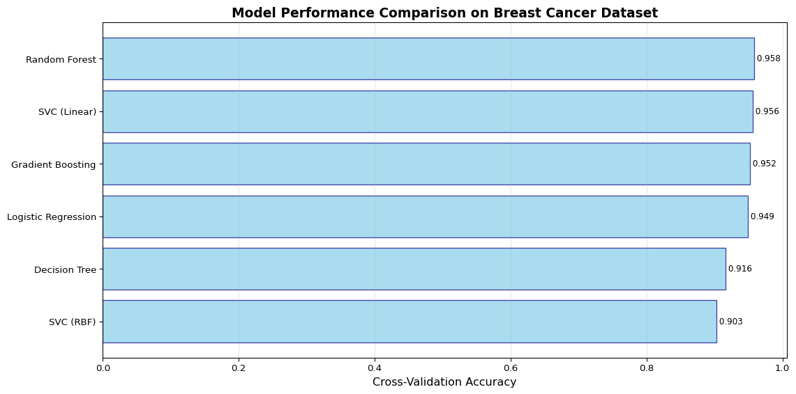
# Create a visualization of model performance
fig, ax = plt.subplots(figsize=(12, 6))

# Sort by accuracy
comparison_sorted = comparison_df.sort_values('accuracy', ascending=True)

# Create horizontal bar plot
y_pos = np.arange(len(comparison_sorted))
ax.barh(y_pos, comparison_sorted['accuracy'],
        align='center', alpha=0.7, color='skyblue', edgecolor='navy')

# Customize plot
ax.set_yticks(y_pos)
ax.set_yticklabels(comparison_sorted.index)
ax.set_xlabel('Cross-Validation Accuracy', fontsize=12)
ax.set_title('Model Performance Comparison on Breast Cancer Dataset', fontsize=14, fontweight='bold')
ax.grid(axis='x', alpha=0.3)

# Add value labels
for i, score in enumerate(comparison_sorted['accuracy']):
    ax.text(score, i, f' {score:.3f}', 
            va='center', fontsize=9)

plt.tight_layout()
plt.show()

print(f"\nBest Model: {comparison_df['accuracy'].idxmax()}")
print(f"Best Accuracy: {comparison_df['accuracy'].max():.4f}")

Figure 1: Model performance comparison on breast cancer dataset


Best Model: Random Forest
Best Accuracy: 0.9582

Example 2.3: Examining All Metrics

# Display all metrics for better comparison
print("\n=== Detailed Metrics for All Models ===")
print(comparison_df.round(4))

# Compare specific metrics
print("\n=== F1 Scores ===")
print(comparison_df[['f1']].sort_values('f1', ascending=False))


=== Detailed Metrics for All Models ===
                     accuracy  precision  recall      f1  roc_auc
Model                                                            
Logistic Regression    0.9495     0.9492  0.9721  0.9602   0.9899
SVC (RBF)              0.9033     0.8827  0.9790  0.9278   0.9686
SVC (Linear)           0.9560     0.9561  0.9756  0.9655   0.9901
Random Forest          0.9582     0.9594  0.9754  0.9671   0.9878
Decision Tree          0.9165     0.9423  0.9266  0.9332   0.9131
Gradient Boosting      0.9516     0.9559  0.9685  0.9619   0.9891

=== F1 Scores ===
                           f1
Model                        
Random Forest        0.967129
SVC (Linear)         0.965453
Gradient Boosting    0.961942
Logistic Regression  0.960232
Decision Tree        0.933165
SVC (RBF)            0.927768

Function 3: `model_evaluation_plotting()`

Purpose

Evaluate a fitted model on test data and generate comprehensive metrics plus confusion matrix visualizations.

Example 3.1: Evaluate Best Model

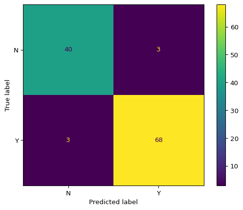
# Use the best estimator from grid search
best_model = best_estimator

# Evaluate on test set
accuracy, f2, y_pred, cm_table, cm_display = model_evaluation_plotting(
    best_model,
    X_test,
    y_test
)

print("\n=== Evaluation Results ===")
print(f"Accuracy: {accuracy:.4f}")
print(f"F2 Score: {f2:.4f}")

print("\n=== Confusion Matrix Table ===")
print(cm_table)

print(f"\n=== Number of Predictions ===")
print(f"Total predictions: {len(y_pred)}")
print(f"Predictions distribution:\n{pd.Series(y_pred).value_counts()}")


=== Evaluation Results ===
Accuracy: 0.9561
F2 Score: 0.9777

=== Confusion Matrix Table ===
col_0   N   Y
row_0        
N      39   4
Y       1  70

=== Number of Predictions ===
Total predictions: 114
Predictions distribution:
Y    74
N    40
Name: count, dtype: int64

Example 3.2: Visualize Confusion Matrix

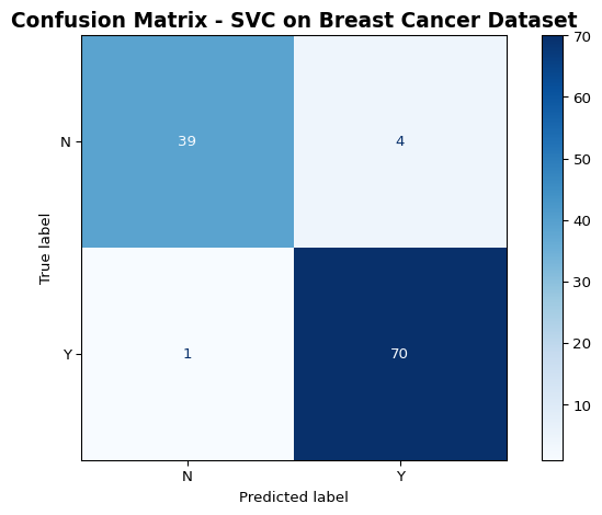
# Display the confusion matrix
cm_display.plot(cmap='Blues')
plt.title('Confusion Matrix - SVC on Breast Cancer Dataset', fontsize=14, fontweight='bold')
plt.tight_layout()
plt.show()

Figure 2: Confusion matrix for breast cancer classification

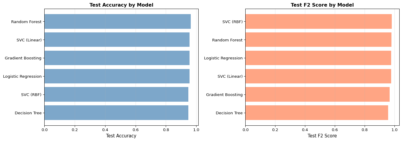
Example 3.3: Compare Multiple Models on Test Set

# Evaluate all models on test set
print("\n=== Test Set Performance Comparison ===")
test_results = []

for model_name, model in models.items():
    # Fit model
    model.fit(X_train, y_train)
    
    # Evaluate
    acc, f2_score, preds, _, _ = model_evaluation_plotting(model, X_test, y_test)
    
    test_results.append({
        'Model': model_name,
        'Test Accuracy': acc,
        'Test F2 Score': f2_score
    })

test_df = pd.DataFrame(test_results).set_index('Model')
test_df = test_df.sort_values('Test Accuracy', ascending=False)
print(test_df.round(4))


=== Test Set Performance Comparison ===
                     Test Accuracy  Test F2 Score
Model                                            
Random Forest               0.9649         0.9804
Logistic Regression         0.9561         0.9777
Gradient Boosting           0.9561         0.9691
SVC (Linear)                0.9561         0.9777
SVC (RBF)                   0.9474         0.9834
Decision Tree               0.9474         0.9577

/opt/buildhome/.local/share/mise/installs/python/3.11.14/lib/python3.11/site-packages/sklearn/linear_model/_logistic.py:406: ConvergenceWarning: lbfgs failed to converge after 1000 iteration(s) (status=1):
STOP: TOTAL NO. OF ITERATIONS REACHED LIMIT

Increase the number of iterations to improve the convergence (max_iter=1000).
You might also want to scale the data as shown in:
    https://scikit-learn.org/stable/modules/preprocessing.html
Please also refer to the documentation for alternative solver options:
    https://scikit-learn.org/stable/modules/linear_model.html#logistic-regression
  n_iter_i = _check_optimize_result(

Example 3.4: Visualize Test Set Comparison

# Create comparison visualization
fig, (ax1, ax2) = plt.subplots(1, 2, figsize=(14, 5))

# Accuracy comparison
test_df_sorted = test_df.sort_values('Test Accuracy', ascending=True)
y_pos = np.arange(len(test_df_sorted))

ax1.barh(y_pos, test_df_sorted['Test Accuracy'], color='steelblue', alpha=0.7)
ax1.set_yticks(y_pos)
ax1.set_yticklabels(test_df_sorted.index)
ax1.set_xlabel('Test Accuracy', fontsize=11)
ax1.set_title('Test Accuracy by Model', fontsize=12, fontweight='bold')
ax1.grid(axis='x', alpha=0.3)

# F2 Score comparison
test_df_f2_sorted = test_df.sort_values('Test F2 Score', ascending=True)
y_pos2 = np.arange(len(test_df_f2_sorted))

ax2.barh(y_pos2, test_df_f2_sorted['Test F2 Score'], color='coral', alpha=0.7)
ax2.set_yticks(y_pos2)
ax2.set_yticklabels(test_df_f2_sorted.index)
ax2.set_xlabel('Test F2 Score', fontsize=11)
ax2.set_title('Test F2 Score by Model', fontsize=12, fontweight='bold')
ax2.grid(axis='x', alpha=0.3)

plt.tight_layout()
plt.show()

Figure 3: Test set performance comparison across models

Complete End-to-End Workflow

Here’s a complete workflow combining all three functions on a fresh dataset:

# Use a subset of features for faster demonstration
from sklearn.datasets import load_iris

# Load Iris dataset
iris = load_iris()
X_iris = pd.DataFrame(iris.data, columns=iris.feature_names)
y_iris = pd.Series(iris.target)

# Convert to binary classification: setosa (0) vs others (1,2)
y_iris_binary = (y_iris != 0).astype(int).map({0: 'N', 1: 'Y'})

X_train_i, X_test_i, y_train_i, y_test_i = train_test_split(
    X_iris, y_iris_binary, test_size=0.2, random_state=42
)

print("=== STEP 1: Compare Multiple Models ===")
iris_models = {
    'Logistic Regression': LogisticRegression(max_iter=1000),
    'SVC': SVC(probability=True),
    'Random Forest': RandomForestClassifier(random_state=42),
    'Decision Tree': DecisionTreeClassifier(random_state=42)
}

iris_comparison = model_cv_metric_compare(iris_models, X_train_i, y_train_i, cv=5)
print(iris_comparison.round(4))

print("\n=== STEP 2: Tune Best Model ===")
# Let's tune the best performing model
best_model_name = iris_comparison['accuracy'].idxmax()
print(f"Tuning: {best_model_name}")

# Tune SVC
svc_param_grid = {
    'C': [0.1, 1, 10],
    'kernel': ['rbf', 'linear'],
    'gamma': ['scale', 'auto']
}

svc_grid = GridSearchCV(SVC(probability=True), svc_param_grid, cv=5, scoring='accuracy')
svc_grid.fit(X_train_i, y_train_i)

tuning_summary, best_svc = param_tuning_summary(svc_grid)
print("\nTuning Results:")
print(tuning_summary)

print("\n=== STEP 3: Final Evaluation ===")
final_acc, final_f2, final_pred, final_cm, final_display = model_evaluation_plotting(
    best_svc,
    X_test_i,
    y_test_i
)

print(f"Final Test Accuracy: {final_acc:.4f}")
print(f"Final Test F2 Score: {final_f2:.4f}")
print(f"\nConfusion Matrix:")
print(final_cm)

=== STEP 1: Compare Multiple Models ===
                     accuracy  precision  recall   f1  roc_auc
Model                                                         
Logistic Regression       1.0        1.0     1.0  1.0      1.0
SVC                       1.0        1.0     1.0  1.0      1.0
Random Forest             1.0        1.0     1.0  1.0      1.0
Decision Tree             1.0        1.0     1.0  1.0      1.0

=== STEP 2: Tune Best Model ===
Tuning: Logistic Regression

Tuning Results:
  Parameter  Value  Best_Score
0         C    0.1         1.0
1     gamma  scale         1.0
2    kernel    rbf         1.0

=== STEP 3: Final Evaluation ===
Final Test Accuracy: 1.0000
Final Test F2 Score: 1.0000

Confusion Matrix:
col_0   N   Y
row_0        
N      10   0
Y       0  20

# Display final confusion matrix
final_display.plot(cmap='viridis')
plt.title('Final Optimized SVC - Iris Binary Classification', fontsize=12, fontweight='bold')
plt.tight_layout()
plt.show()

print("\n=== Workflow Complete! ===")

Figure 4: Final model confusion matrix on iris dataset


=== Workflow Complete! ===

Summary

You’ve learned how to:

Extract hyperparameter tuning results with param_tuning_summary()
Compare multiple models efficiently with model_cv_metric_compare()
Evaluate and visualize results with model_evaluation_plotting()
Combine all functions in an end-to-end ML workflow

Next Steps

Explore the API Reference for detailed function signatures
Check out the GitHub repository for source code
Report issues or contribute via our Issue Tracker
Read Contributing Guidelines to contribute to the project

Tips for Best Results

Always use pandas DataFrames for X and pandas Series for y
Ensure models are fitted before using model_evaluation_plotting()
This package requires binary classification with labels “Y” and “N”
For models that support it, enable probability=True for SVC to compute ROC-AUC scores
Consider computational cost when setting parameter grids for tuning

Introduction

Setup and Data Loading

Function 1: param_tuning_summary()

Purpose

Example 1.1: GridSearchCV with SVC

Example 1.2: RandomizedSearchCV with Random Forest

Key Outputs

Function 2: model_cv_metric_compare()

Purpose

Example 2.1: Basic Model Comparison

Example 2.2: Visualizing Comparison Results

Example 2.3: Examining All Metrics

Function 3: model_evaluation_plotting()

Purpose

Example 3.1: Evaluate Best Model

Example 3.2: Visualize Confusion Matrix

Example 3.3: Compare Multiple Models on Test Set

Example 3.4: Visualize Test Set Comparison

Complete End-to-End Workflow

Summary

Next Steps

Tips for Best Results

Function 1: `param_tuning_summary()`

Function 2: `model_cv_metric_compare()`

Function 3: `model_evaluation_plotting()`